


I’ll show you the weighted average formula, how it calculates, and I’ll prove that the answer is correct!
(Download my Excel file)
Weighted Average Formula
Column B has the count. Column C has the weight. Weighted average formula is:
=SUMPRODUCT(B2:B12,C2:C12)/SUM(B2:B12)
12.05 is the answer.

Pic 1
Why Weighted Average?
Pic 2
Why can’t we just use a normal average?
If we average the numbers in column C we get an average of 14.0
BUT….it wouldn’t fairly represent our group of dogs.
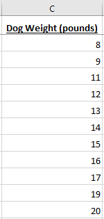
Look at Pic 1, does an average of 14.0 look right???
Remember: 1 dog weighs 8 pounds, 7 weigh 9 pounds, 10 weigh 11 pounds, 11 weigh 12 pounds etc.
=AVERAGE(C2:C12) ignores the fact that most dogs weigh 9, 11, or 12 pounds (that’s 28 of 40 dogs). Only 7 dogs weigh 14 or more pounds.
Column D below helps to visualize this. I changed the font size to reflect their weight.
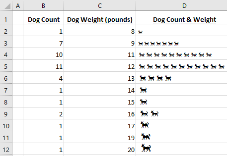
Pic 3
Weighted Average Logic
This is our weighted average formula:
=SUMPRODUCT(B2:B12,C2:C12)/SUM(B2:B12)
Let’s examine each part separately:
SUMPRODUCT(B2:B12,C2:C12)
SUMPRODUCT does this (1 dog X 8 pounds) + (7 dogs X 9 pounds) + (10 dogs X 11 pounds) etc =482
SUM(B2:B12)
SUM is simply counting the dogs. =40
SUMPRODUCT (482) divided by SUM (40) gives us the correct weighted average of 12.05
Weighted Average Proof!
We were given the summary of the original data(Pic 1). Let’s recreate the data!
Step 1 Cumulative Sum: column A has a cumulative sum (+1) of column B dog count values. This creates binning groups.
Step 2 Counter: a sequential counter from 1 to 40 (40 dogs). Represents dog #1, dog #2, dog #3, etc.
Step 3 Binning: =MATCH(M2,$A$1:$A$13,TRUE) finds each counter value in column A. TRUE (approximate match) not FALSE (exact match) bins each counter number.
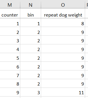
Pic 4
Pic 4 shows that dog #1 weighs 8 pounds. Dogs 2,3,4,5,6,7,8 all weigh 9 pounds (group or bin 2).
Look at counter value of 9. Dog #9 falls into bin 3 and has a weight of 11 pounds.
The Proof: Use the normal average on column O. It’s the same as the weighted average!
Dog Histogram

How did I create it?
I used formula =REPT(“õ”,B2)
Cell font = Webdings
I manually changed the font size (vba would be better!)
My inner nerd took over my body:
I changed the formula to: =REPT(VLOOKUP($V$1,’Animal List’!$A$2:$B$5,2,0),B2)
In cell V1 select from a list (maybe you have pet squirrels !!)
NOTE: if you increase the dog counts in column B then extend formulas in columns M,N, and O.
Weighted Average Video
Watch this video from Microsoft.
My Dogs
Cali (on the right) weighs 10 pounds and Fenton weighs approximately 14 pounds (he wiggles a lot on the scale at the vet).

That’s me in the middle. I weigh a lot more! My name is Kevin Lehrbass. We live in Markham Ontario Canada.
I’ve been a Data Analyst since 2001. Microsoft Excel is my favorite software but Cali & Fenton get mad at me if I spend too much time in Excel.
Their hobbies: getting treats, barking at squirrels, naps with me on the couch.