Standard Deviation in Excel

How tall is tall? How smart is smart? How do we compare? Normal Distribution and Standard Deviation answer this. We’ll review the concepts and use Excel to crunch the numbers.

How Do We Compare?

Numbers describe height, intelligence and tests. How do we compare these numbers to others?

Tim is 2 meters tall! That’s extremely tall!
Sonja’s IQ is 117. She’s a genius!
I got 76% on the test. Not bad.

We’ll use height. Normal Distribution & Standard Deviation allow us to compare height.

Why Height?

It’s easier to visualize than test scores or IQ. In a crowd you compare the height of those around you. Internally you do the math.

Bill Jelen (Mr Excel) and I in 2015.

Bill is 6 feet 1 inch (185 cm). I am 6 feet 4 inches (194 cm).

Instead of using adjectives to describe our height we’ll use standard deviations.

Normal Distribution

What do height, I.Q. and test scores have in common? All are normally distributed.

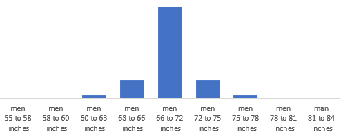
Chart below shows: most are close to the mean(average), half are above the mean and half are below.

Some are taller (to the right) or shorter (to the left). Very few are extremely tall or short.

In the U.S. average male height is 5 feet 9.3 inches (69.3 inches, 176 cm). source

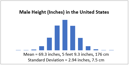
Left and right sides of the chart are symmetric. Normally distributed data-sets share this symmetry but the spread varies. Values may cluster around the mean or be more spread out. Standard deviation measures this. Normal distribution is also known as Gaussian distribution and the bell curve.

Standard Deviation

Measures the spread of the numbers from the average (mean) in normally distributed data-sets.

68.27% of values are within one standard deviation of the mean.
95.45% of values are within two standard deviation of the mean.
99.73% of values are within three standard deviation of the mean.

It works for all normally distributed data-sets. In statistics this is known as the empirical rule.

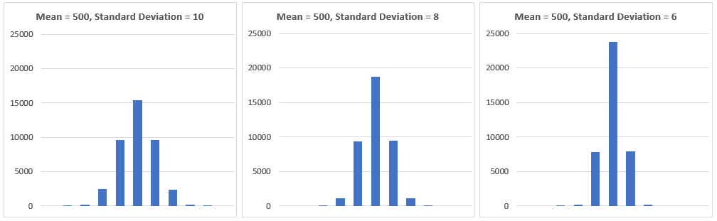
Data clusters closer to the mean as standard deviation decreases. The empirical rule still works.

For U.S. male height 1 standard deviation = 2.94 inches (7.5 cm). Let’s explore this in Excel!

Excel Sample Data-set

In sheet ‘INPUTS & DATA’ I created a sample date-set using:

mean male height of 5 feet 9.3 inches (69.3 inches, 176 cm)
standard deviation of 2.94 inches (7.5 cm)
formula in column E =NORM.INV(RAND(), 69.3, 2.94) (pasted as values)

Below we see the sample of 30000 produced results very close to the empirical rule.

20510 (68.37%) within 1 stand dev of mean (66.37 to 72.24 inches, 68.57 to 183.49 cm)
28618 (95.39%) within 2 stand dev of mean (63.43 to 75.18 inches, 61.11 to 190.95 cm)
29932 (99.77%) within 3 stand dev of mean (60.49 to 78.11 inches, 53.65 to 198.41 cm)

Displayed using feet and inches:

68.37% are between 5 feet 6 inches and 6 feet 0 inches.
95.39% are between 5 feet 3.4 inches and 6 feet 3.2 inches.
99.77% are between 5 feet 0 inches and 6 feet 6 inches.

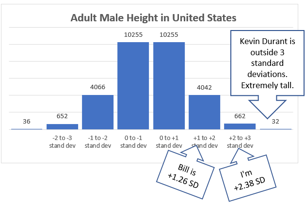
Bill’s 1.26 standard deviation is between the 1st & 2nd deviation above the mean.

My 2.38 standard deviation is between the 2nd & 3rd deviation above the mean.

Men above 6 feet 6 inches (past 3rd standard deviation) are extremely tall. Kevin Durant is 6 feet 11 inches with a standard deviation of 4.7

Comparing to Other Countries

This entire post I’ve been referring to male height in the United States.

What if Bill and I were to travel to Bolivia? Would we be taller?

Of course not but we’d be perceived as being taller by the local people! In Bolivia my height would put me 4.5 standard deviations above the 5 feet 3 inch mean (2.92 inch SD). Bill would be 3.4 standard deviations above the mean. If we traveled to The Netherlands my standard deviation would be 1.7 and Bill’s would be 0.6. We would blend in quietly. Isn’t that weird?

What is Skew?

If a data-set is perfectly symmetrical (left side of chart is exactly like right side) the skew is zero.

Our sample of 30000 gave us a skew of 0.00561 Closer to zero means more symmetrical.

In sheet ‘STATS’ row 26 I calculate the skew for various small samples.

skew = -0.6108 (10 rows of sample data)
skew = -0.1818 (100 rows of sample data)
skew = -0.0972 (1000 rows of sample data)
skew = 0.0072 (10000 rows of sample data)

The skew decreases as we include more data! If a data-set is truly normally distributed the skew approaches zero as the sample increases.

?Mean = Median?

In sheet ‘STATS’ rows 23 & 24 we see the mean and median values for the small samples. Row 25 shows that the absolute difference decreases as we include more sample data!

The mean and median values get closer and closer as we increase the sample size.

0.832 absolute difference (10 rows of sample data)
0.169 absolute difference (100 rows of sample data)
0.041 absolute difference (1000 rows of sample data)
0.026 absolute difference (10000 rows of sample data)

Chart Tricks

Horizontal axis labels are linked to cells I14:I22 (sheet STANDARD DEVIATION CHART).

To get the right look and functionality I used three chart tricks.

(1) They weren’t displaying properly (text was jammed together)

To fix this I forced two carriage returns using the CHAR function. Character 10 does the magic. Now the text displays nicely in three lines.

(2) I wanted a way to easily switch between metric and imperial

I added a check box (check = metric, uncheck = imperial) and used the TRUE FALSE in the formula.

(3) I only wanted to display the integer (not all the decimals)

I used the TEXT function to format the number. I also could have used the FLOOR function.

The end formula is a bit long but it gets the job done:

=IF(H13=0,””,IF(H13=1,”man “,”men “)&CHAR(10)&IF($J$12,TEXT(F12,0)&” to “&TEXT(F13,0)&CHAR(10)&” inches”,TEXT(G12,0)&” to “&TEXT(G13,0)&CHAR(10)&” cm”))

Excel File

Download my Excel file. There are 5 sheets:

INPUTS & DATA enter parameters to create data-set
PIVOT TABLE & CHART summarize & visualize
STANDARD DEVIATION CHART visualize by standard deviations
STATS additional statistics
HEIGHT EXAMPLES used in this post

To see how to create the sample data you can replace the pasted values in column E sheet INPUTS & DATA) with formula =NORM.INV(RAND(), $B$5, $B$8)

About Me

My name is Kevin Lehrbass. I’m a Data Analyst.

Normal stores rarely sell my pant size. L.L. Bean’s catalog used to have my size but not any more. Big & Tall stores say “we don’t have that small size” or they do but a single pair costs a fortune.

That day I did find my size and there was a sale! I bought all the pairs they had in stock!

The site is about Microsoft Excel.