


For Mr Excel’s recent challenge I decided to go with an old school formula helper column solution. Why? I’ll explain.
Excel file (original file from Bill Jelen) used in this post (read his original post).
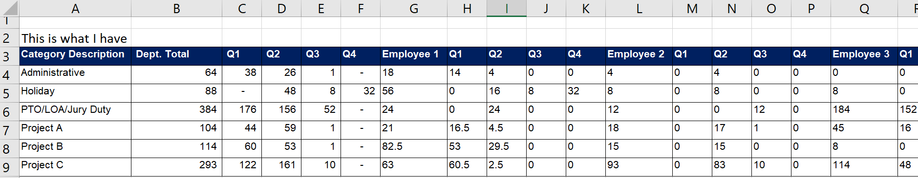
The Challenge
Someone attending one of Bill’s training sessions had this data-set:
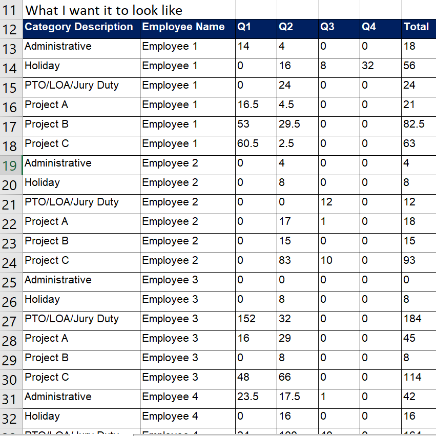
…and needed to rearrange it into this:
Power Query?
Yes, it’s an amazing way to solve this but it requires a refresh if your data changes. Great thing about PQ is that it does all the work and drops the finished dataset back into a sheet (no formulas that need calculating). Nevertheless, I went old school with a formula helper column solution 🙂
Formula Helper Columns
Years back I’d often build a single monster array formula to solve something like this. Nowadays I prefer to break down a solution into a series of helper formulas that are easier to audit and explain to others.
Getting Started
My Excel file (original file from Bill Jelen) also contains an explanation.
Key question for re-arranging data: What’s the pattern?
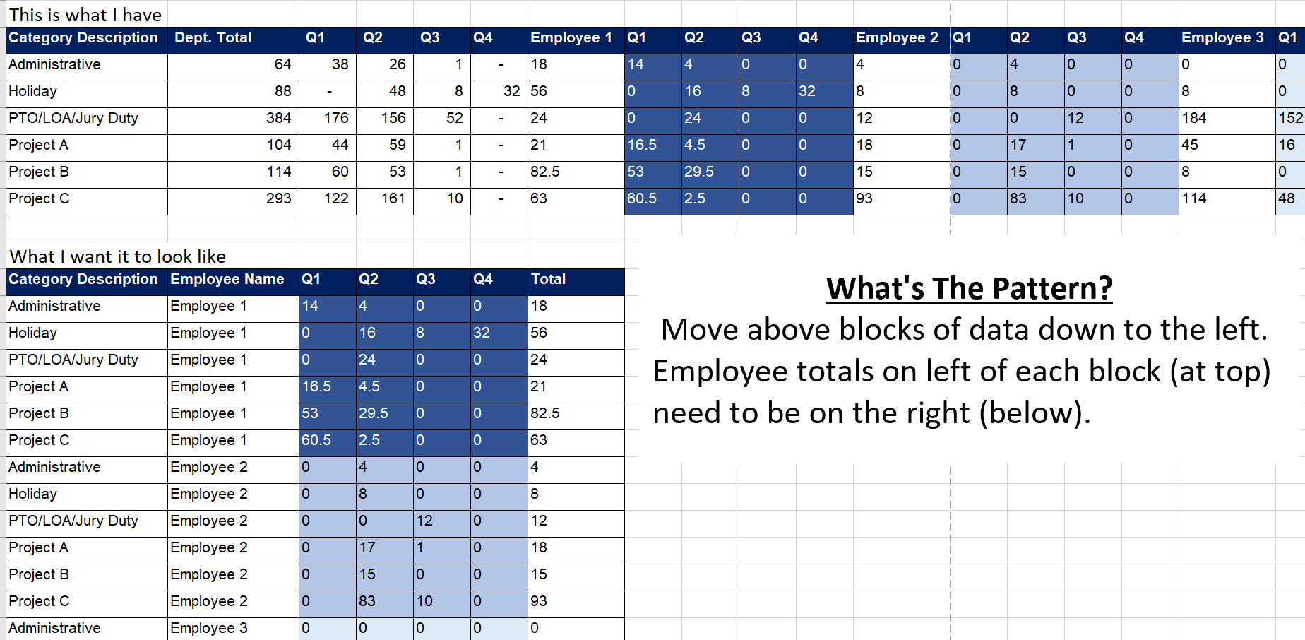
Each data block at the top (moving right) is to be stacked below. Total columns above, below each employee name and to the left of each block, need to be to the right of each block below.
Before we create formulas to get these blocks let’s create formulas to display Category & Employee.
Category & Employee
For each data block we need to repeat ‘Category Description’ and ‘Employee Name’ multiple times.
Each one has 2 formulas: 1) helper that defines the position, 2) index function gets the answer.
This is the Category helper column:
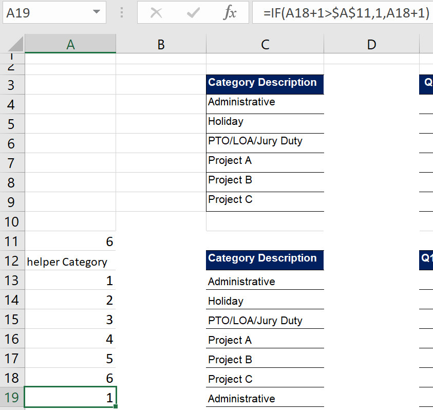
There are 6 categories (cells C4 to C9).
Column A helper formula is a simple way to repeat sets of 1 to 6.
Simple Index function in column C uses this helper to get the category.
This is the Employee helper column:
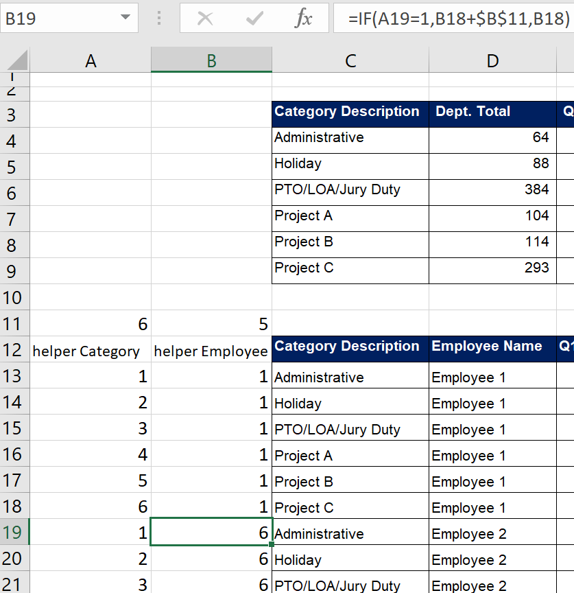
Column D has this formula:
=INDEX($I$3:$AB$3,$B19)
It slides right along row 3 to get the Employee’s name.
Now it’s time to get the data!
Get the Data
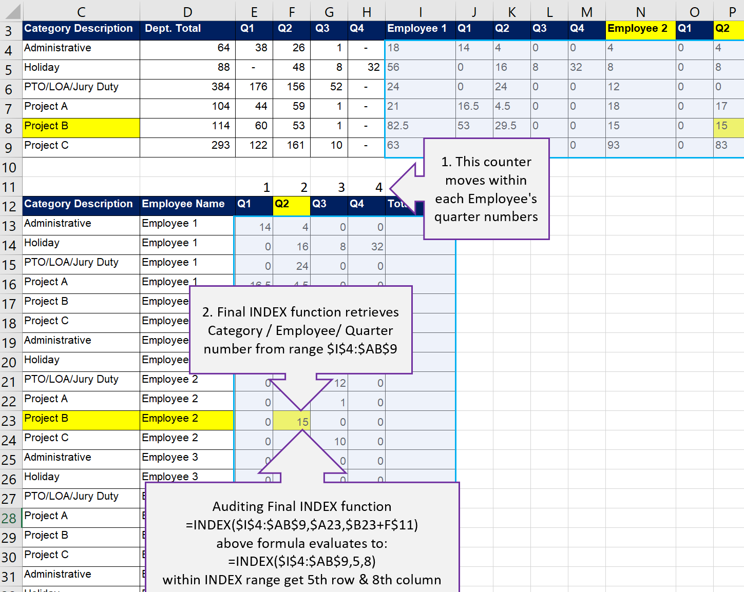
Let’s look at cell F23. Formula is =INDEX($I$4:$AB$9,$A23,$B23+F$11)
We reuse helper values from columns A & B and the values in row 11.
Index range $I$4:$AB$9 has all answers.
$A23 = 5 (5th item down = “Project B”). $B23+F$11 = 8 (8th item across = “Q2”).
The intersection of 5th item down & 8th item across = 15 (yellow below).
Verify Results
Normally we wouldn’t have the desired result (sheet ‘original’). So, my formula in cell M12 of sheet ‘FINAL’ wouldn’t work.
A simple way to check results is to change a value at the top (original layout) and ensure that it changes below (desired layout). This is especially helpful if the data has low cardinality (many repeat values). Obviously you would change the value back to it’s original value after verifying it.
Recap
Splitting the solution into various helper formulas makes it easier to explain, audit and adjust. In rare cases I still use megaformulas (formula with numerous functions) but my advice is to be kind to others and also your future self by creating solutions that won’t cause pain and suffering. My solution is also backwards compatible.
Mr Excel’s Video & Post
Here is Bill’s original video that introduces the challenge. His summary post has links to the different groups of solutions (i.e. formula solutions).
Bill Jelen (Mr Excel) declares Bill Szysz’s Power Query solution the winner!
Don’t forget to visit Mr Excel’s Message Board where a team of volunteers answer your Excel questions for free!
About Me

That’s me Kevin Lehrbass on the left and Bill Jelen (Mr Excel) on the right.
I’m a Data Analyst. I live in Markham Ontario Canada (near Toronto).
This is my personal blog about Microsoft Excel. Here’s a previous post of mine that’s also about re-arranging data.