


Robert Gascon not only created a shortest formula challenge but he also challenged me to write a post about it!
The Challenge
Here’s the link to Robert’s shortest formula challenge.
Understanding The Challenge
I initially struggled to understand it. Maybe that’s part of the challenge! On my 3rd attempt I got it!
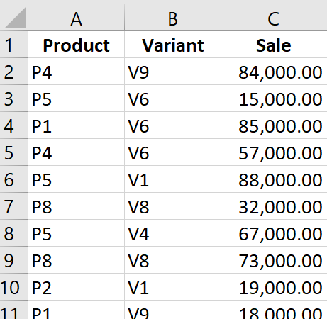
Raw Data
Three columns of raw data in columns A, B, and C. 119 rows of data.
Multi-step Solution
Starting in cell E1 we see 8 different matrices. Various combinations of Products (column A) and Variants (column B). Let’s focus on the top matrix (challenge #1).
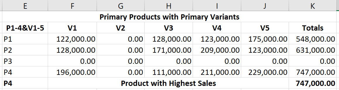
- SUMIFS, range F3:J6, sum column C based on product and variant conditions
- Column K has a total for each row
- Cell K7 MAX function displays max value from totals above
- “P4” has max total row of 747000. Cell E7 lookup function = “P4” (max total of items P1 P2 P3 P4)
The Challenge
Scroll down to row 70 to see challenge #1.
Cell J70 shows answer “P4” by referencing cell E7 that we just saw. Here’s the challenge:
For challenge #1 get answer “P4” using a single formula!
I’m won’t attempt to solve this. My victory is understanding Robert’s solution!
Robert’s Formula Solution
Cell K70 has Robert’s formula solution for challenge #1:
=LOOKUP(2,
1/FREQUENCY(0,1/(1+MMULT(SUMIFS(C$2:C$120,
A$2:A$120,”P”&ROW($1:$4),B$2:B$120,”V”&COLUMN(A:E)),
ROW($1:$5)^0))),
“P”&ROW($1:$4))
LOOKUP function has 3 parts. Part 1 and part 3 are simple. Part 2, lookup_vector, is the beast!
LOOKUP(lookup_value, lookup_vector, [result_vector])
Sneaky Concept
lookup_value of 2 will never be found in the lookup_vector. Huh? I’ll explain:
I’ve evaluated (using F9 key) lookup_vector and [result_vector]. Results are:
=LOOKUP(2,
{#DIV/0!;#DIV/0!;#DIV/0!;1;#DIV/0!},
{“P1″;”P2″;”P3″;”P4”})
2 isn’t found in the lookup_vector . 1 is the only number in lookup_vector.
If the only number is equal to or less than the lookup_value the function can return the [result_vector] answer. As the lookup_vector 1 is in the 4th position the [result_vector] gives us “P4”.
Let’s modify it a bit:
=LOOKUP(2,
{1;#DIV/0!;#DIV/0!;#DIV/0!;#DIV/0!},
{“P1″;”P2″;”P3″;”P4”})
Now the answer is “P1”.
=LOOKUP(2,
{#DIV/0!;2;3;3;4;#DIV/0!},
{“P1″;”P2″;”P3″;”P4”})
Answer is “P2”. Ok…let’s move on.
The Brain
lookup_vector is the brain of Robert’s solution:
1/FREQUENCY(0,1/(1+MMULT(SUMIFS(C$2:C$120,
A$2:A$120,”P”&ROW($1:$4),B$2:B$120,”V”&COLUMN(A:E)),
ROW($1:$5)^0)))
Inside SUMIFS he has used ROW and COLUMN to create the “P” and “V” values:
Select criteria1 “P”&ROW($1:$4) and press F9 key to see: {“P1″;”P2″;”P3″;”P4”}
Select criteria2 “V”&COLUMN(A:E) and press F9 key to see: {“V1″,”V2″,”V3″,”V4″,”V5”}
SUMIFS looks like this:
SUMIFS(C$2:C$120,
A$2:A$120,{“P1″;”P2″;”P3″;”P4”},B$2:B$120,{“V1″,”V2″,”V3″,”V4″,”V5”})
Let’s audit MMULT function using the F9 key to see the results:

Using F9 on MMULT’s array1 and array2 gives us:
=LOOKUP(2,
1/FREQUENCY(0,1/(1+MMULT({122000,0,128000,123000,175000;128000,0,171000,209000,123000;0,0,0,0,0;196000,0,111000,211000,229000},{1;1;1;1;1}))),
“P”&ROW($1:$4))
Examine the numbers inside MMULT. They are the same numbers found in range F3:J6 !MAGIC!
…the final result of MMULT is:
=LOOKUP(2,
1/FREQUENCY(0,1/(1+{548000;631000;0;747000})),
“P”&ROW($1:$4))
Notice something? {548000;631000;0;747000} are total column numbers from range K3:K6 !MAGIC!
and now evaluate what FREQUENCY function does:
=LOOKUP(2,
1/FREQUENCY(0,1/{548001;631001;1;747001}),
“P”&ROW($1:$4))
…eventually becomes this:
=LOOKUP(2,
1/{0;0;0;1;0},
“P”&ROW($1:$4))
and then:
=LOOKUP(2,
{#DIV/0!;#DIV/0!;#DIV/0!;1;#DIV/0!},
“P”&ROW($1:$4))
As Robert says in his comment below, FREQUENCY function returns the maximum of the row totals.
Summary
F9 key is your best friend. Use it until you see how Robert gets the same result but in only 1 formula. I just realized that it’s 10pm and I forgot to eat supper. Who needs food when you have an interesting formula to audit 🙂
Thank You
A special thanks to Robert Gascon for this interesting Excel challenge. We need these kinds of distractions these days.
As amazing as Robert’s formula solution is there’s no way I’m going to attempt to create a shorter solution! Is it possible? Maybe…but I’ll let others try.
Follow Robert’s contributions to Microsoft Tech Community: https://techcommunity.microsoft.com/t5/user/viewprofilepage/user-id/280482
Hi Kevin,
You had an amazing analysis, as usual. Let me emphasize that I used MMULT to return the sum for each row or column, and FREQUENCY to return the maximum of the sums.
Cheers,
Robert
That’s a good point. I made some additions/changes to the post to clarify.
Thanks Robert!!
Dear Robert H. GASCON
Please, if it’s possible share the excel file with your formula.
Best regards,
Tehrani
[email protected]
Hi Hamid,
You should be able to get the Excel file here: https://techcommunity.microsoft.com/t5/excel/shortest-formula-challenge/m-p/1660217
Thanks for visiting my blog.
Cheers,
Kevin
Hi Hamid,
I already attached the solution file here:
https://techcommunity.microsoft.com/t5/excel/shortest-formula-challenge/m-p/1951063#M82725
I do not know where you found his formula, but if it is truly about the shortest formula, and if the only rules to follow are the stated rules — i.e. if we can use things like ROW(1:4) instead of ROW($1:$4) — then I think we can drop some dollar signs as well as using MATCH instead of LOOKUP to get a formula that is 16 characters shorter.
=”P”&MATCH(1,FREQUENCY(0,1/(1+MMULT(SUMIFS(C$2:C$120,A$2:A$120,”P”&ROW(1:4),B$2:B$120,”V”&COLUMN(A:E)),ROW(1:5)^0))),0)
And for any of the “secondary” challenges, just add the appropriate number to the MATCH result — e.g. use +5 on Challenge #4 since it begins with V6.
Of course I also think Robert’s solution could have been 2 characters shorter by looking for a 1 instead of 2 and dropping the extra 1/ to have this instead:
=LOOKUP(1,FREQUENCY(0,1/(1+MMULT(SUMIFS(C$2:C$120,A$2:A$120,”P”&ROW($1:$4),B$2:B$120,”V”&COLUMN(A:E)),ROW($1:$5)^0))),”P”&ROW($1:$4))
And if the same dollar signs were dropped here as well, then the MATCH version only wins by 8 characters. Regardless, it is the FREQUENCY trick that is the true genius of the solution.
Hi David,
I found Robert’s formula here: https://techcommunity.microsoft.com/t5/excel/shortest-formula-challenge/m-p/1660217
Thanks for your comment and visiting my blog. I’ll have to slowly and carefully study your modifications to the formula. Yes, the FREQUENCY function trick is definitely the genius of Robert’s solution. I really had to focus to understand it.
Seems you are one of those people like Robert and I that finds Excel endlessly fascinating! Robert and I have also done some posts on the combination of Chess and Excel that were a lot of fun!
https://www.myspreadsheetlab.com/excel-chessgames-viewer/
https://www.myspreadsheetlab.com/chess-fen-viewer/
Cheers,
Kevin
Apparently Robert’s formula can’t be shortened by two characters as I thought because that variation won’t work with challenge #7 even though I can’t figure out why.
I’m definitely someone with an endless Excel fascination. I like your chess examples, and although I haven’t yet explored them fully, I can offer one suggestion. I still have Excel 2013 on my current computer, so I can’t take full advantage of TEXTJOIN, but I’m pretty sure it could be used along with the following formula as one way to shorten your approach to the FEN Viewer (less helper columns, probably cutting out at least steps 2 through 5):
=REPT(MID(P7,ROW($A$1:INDEX(A:A,LEN(P7))),1),IFERROR(VALUE(MID(P7,ROW($A$1:INDEX(A:A,LEN(P7))),1)),1))
In fact, you could probably eliminate all of the helper columns by the time you’re done.