Earlier this week I saw an interesting rounding question on the famous MrExcel Forum. And there was a twist!

Excel File

Download the Excel file and follow along.

Original Question

Link

Link to the original post on MrExcel’s amazing AND free help forum.

Description

I created this Excel file to explain:

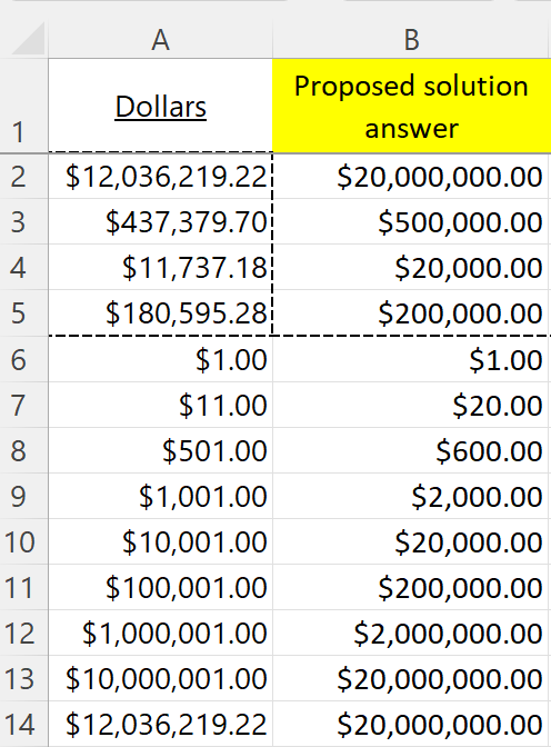
Original values in cells A2:A5 (I added more below). Solution in column B.

Solution

Cell B2 formula:

=ROUNDUP(A2,-INT(LOG10(A2)))

A brilliant formula from one of the forum members. It rounds like this:

• $12,036,219.22 to $20,000,000.00
• $437,379.70 to $500,000.00

The Twist

Twist Definition

$12,036,219.22 (numbers with 8 digits to the left of decimal) should round to $13,000,000.00 (not $20,000,000.00). This is the only exception.

Twist Solution 1

With only 1 exception why not use the IF function? Formula in cell D2:

=ROUNDUP(A2,IF(-INT(LOG10(A2))=-7,-6,-INT(LOG10(A2))))

-INT(LOG10(A2)) determines the rounding level. IF function tests for the exception changing rounding level only for the exception.

Twist Solution 2

Multiple exceptions? How can I make it easy to modify them?

=ROUNDUP(A2,INDEX(list!$B$1:$B$8,MATCH(-INT(LOG10($A2)),list!$A$1:$A$8,0)))

Formula looks into column A and retrieves desired rounding level in column B. It’s easy to change rounding level in column B.

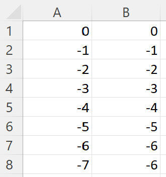
Note: cell A8 value of -7 is the exception. It rounds to -6 (not -7).

Twist Solution 3

Can I remove the lookup table? I created this:

=ROUNDUP(A2,INDEX({0;-1;-2;-3;-4;-5;-6;-6},MATCH(-INT(LOG10($A2)),{0;-1;-2;-3;-4;-5;-6;-7},0)))

It uses two array constants instead of a lookup table.

Modify desired rounding levels inside INDEX function as needed: INDEX({0;-1;-2;-3;-4;-5;-6;-6}

Creating an Array Constant

Twist Solution 3 has two array constants. I could type values directly in the formula but the syntax is tricky. I modified Twist Solution 2 formula.

Twist Solution 2:
=ROUNDUP(A2,INDEX(list!$B$1:$B$8,MATCH(-INT(LOG10($A2)),list!$A$1:$A$8,0)))

--see "5 Steps..." further down to convert formula Twist Solution 2 into formula Twist Solution 3:

Twist Solution 3:
=ROUNDUP(A2,INDEX({0;-1;-2;-3;-4;-5;-6;-6},MATCH(-INT(LOG10($A2)),{0;-1;-2;-3;-4;-5;-6;-7},0)))

5 Steps to convert sheet list references into array constants:

1. in formula bar highlight list!$B$1:$B$8
2. press F9 key (on laptop: hold Fn key then press F9 key) to hard code values
3. still in formula bar highlight list!$A$1:$A$8
4. press F9 key (on laptop: hold Fn key then press F9 key) to hard code values
5. press Enter key (to permanently hard codes values)

The formula should now look like this:

=ROUNDUP(A2,INDEX({0;-1;-2;-3;-4;-5;-6;-6},MATCH(-INT(LOG10($A2)),{0;-1;-2;-3;-4;-5;-6;-7},0)))

Finally, show a co-worker your amazing formula 🙂

MrExcel Help Forum

Bill Jelen (aka MrExcel) created his forum over 20 years ago. It’s an incredible free source to answer Excel related questions. Bill also writes/publishes books, offers consulting services, and has a popular YouTube channel.

About Me

I’m a Data Analyst and major Excel fan. I live in Markham Ontario Canada.