

I enjoy the dueling Excel podcasts between Bill Jelen and Mike Girvin! The challenges, the energy, the solutions, the community involvement…everything! Let’s look at Excel duel 141 (the PI episode). The best solution depends on asking one question.
The Excel Legends!
Mike Givin and Bill Jelen (video links are below).

The Challenge
There are three numbers. We need to:
- lookup each number into a different lookup table
- return the Mult Factor found to the right
- multiply the three answers
The Data
Andy met 0 goals in Category 1, 5 goals in Category 2 and 2 goals in Category 3.

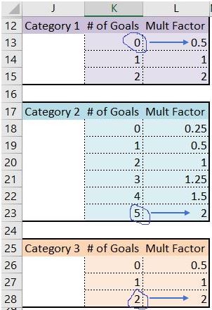
Below we see the three lookup tables. We need to return the ‘Mult Factor‘ for each value.
Andy’s 0 = 0.5, his 5 = 2, his 2 = 2.
0.5 X 2 X 2 = 2!
The Question
This key question makes a big difference:
WILL YOU ALWAYS HAVE ONLY THREE CATEGORIES?
Remember, we want to solve it not over-solve it !
If you’ll always have three (or maybe a couple more) you can use a simple solution.
If you could have many categories (i.e. 50) then a more dynamic solution is worth the effort.
simple solution
If only a limited number of categories it can be solved quickly and explained to anyone!
Bill Jelen (Mr Excel) solved it using three VLOOKUP functions!
=VLOOKUP(B8,$K$13:$L$15,2,0)*VLOOKUP(C8,$K$18:$L$23,2,0)*VLOOKUP(D8,$K$26:$L$28,2,0)
Mike Girvin (ExcelisFun) solved it using three LOOKUP functions! It works as data is sorted.
=LOOKUP(B8,$K$13:$L$15)*LOOKUP(C8,$K$18:$L$23)*LOOKUP(D8,$K$26:$L$28)
dynamic solutions
If there could be let’s say 50 categories then we know we can’t fit 50 vlookups into a cell.
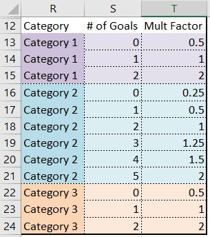
Put all the data together! Simply add more categories below. If you’re not afraid of tables then select anywhere inside of the data, hold ‘Ctrl’ key and press ‘T’ (to create a table). If you use a table then you don’t have to adjust your formula ranges.
Array Solution by XLarium
One array formula solves it!
To enter an array hold ‘Ctrl’ and ‘Shift’ keys and then press ‘Enter’ key (instead of just pressing ‘Enter’).
=PRODUCT(IF($R$13:$R$24=$B$7:$D$7,IF($S$13:$S$24=B8:D8,$T$13:$T$24)))
This array was created by “Xlarium“. He is awesome!
How does the array work?
Inside the PRODUCT function the goal is to extract 3 ‘Mult Factor’ numbers (as we have 3 categories).
IF($R$13:$R$24=$B$7:$D$7 normally an array condition is a single value. Here, we have $B$7:$D$7 (all 3 categories).
IF($S$13:$S$24=B8:D8 the 2nd condition filters to the goals that Andy achieved (0, 5 and 2).
$T$13:$T$24 qualifying answers (o.5, 2, 2) are taken from ‘Mult Factor‘ column and multiplied because the array is wrapped with the PRODUCT function.
Array Solution by me 🙂
My solution uses a lookup function wrapped with the product function (as the lookup returns 3 answers it needs C.S.E.)
No conditions are required in the array but there is a helper column called ‘Key’.
Excel Files
Mike Girvin posts all of his amazing Excel files here. Or use the direct link here for trick 141.
Here is the Excel file I used that’s based on the file from Mike and Bill.
YouTube Videos
Mike Girvin’s video. Bill Jelen’s video.
PI Reference?
Today is PI day (March 14 = 3.14). Download my Excel file to see my PI formula. I admit it’s rather lame but it works!
About Me

My name is Kevin Lehrbass. I’m holding my dogs Fenton and Cali. I’ve been a data analyst since 2001. Wow…time flies!
I’m still learning! I’m studying Power Query Academy! created by Ken Puls & Miguel Escobar. Also, see my recommended training.
DISCLAIMER: i’m an affiliate for these courses.
Thanks for digging up that old duel video and mentioning, Kevin.
Hi XLarium. You’re welcome! Your array solved it so quickly! Thanks for reading!
Cheers,
Kevin
Hello Kevin,
This is my favorite among your posts in 2018. As usual, I use my favorite LOOKUP function. Here is my non-array formula in Cell T8, copied down to Cell T10:
=PRODUCT(INDEX(LOOKUP(B$7:D$7&B8:D8,
R$13:R$24&S$13:S$24,
T$13:T$24),0))