


My friend Robert Gascon was thinking about Excel formula challenges and Kentucky Fried Chicken (he loves KFC) while drinking a beer.
Formula Challenge!
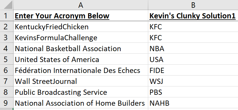
Robert realized KFC Kentucky Fried Chicken = KFC Kevin’s Formula Challenge
He then described the challenge:
Using formulas, create KFC out of Kentucky Fried Chicken.
It’s an acronym creator. Shortest formula wins!
Challenge Details
I might have to add more rules later to clarify but let’s start with:
- extract only upper case letters
- each word starts with upper case letter
- each word has only one upper case letter
- text may or may not have spaces
- no accents on upper case letters
- sheet name is “x” (only 1 character)
- length must = count of upper case letters
- shortest formula wins
I later realized that there are 2 variations of this challenge:
- text contains only letters (upper & lower) and spaces
- text contains any kind of characters
If the text could contain any kind of character then the solution needs to be more robust.
Download my Excel file.. Post your formula as a comment below.
Kevin’s Solutions
I came up with 3 solutions. Can you create a shorter solution?
Here’s my 1st formula. It’s 182 characters long:
=SUBSTITUTE(CONCAT(CHAR(IF((CODE(MID(A2,ROW(INDIRECT(“1:”&LEN(A2))),1))>64)
*(CODE(MID(A2,ROW(INDIRECT(“1:”&LEN(A2))),1))<91),
CODE(MID(A2,ROW(INDIRECT(“1:”&LEN(A2))),1)),
91))),”[“,””)
My 2nd formula is 140 characters long:
=SUBSTITUTE(CONCAT(IFERROR(CHAR(IF(CODE(MID(A2,ROW(INDIRECT(“1:”&LEN(A2))),1))
<91,CODE(MID(A2,ROW(INDIRECT(“1:”&LEN(A2))),1)))),””)),” “,””)
Normally, array formulas require Control Shift Enter. The { } array brackets. However, I have the new version with dynamic arrays. My formula works without Control Shift Enter. I save two characters!
Cheating?
My 3rd solution is the shortest but is it cheating?
Notice that in the formulas above I had to use this part twice:
=CODE(MID(x!A2,ROW(INDIRECT(“1:”&LEN(x!A2))),1))
So…I put this part in a named range called z. Now my formula is reduced to:
=SUBSTITUTE(CONCAT(IFERROR(CHAR(IF(z<91,z)),””)),” “,””)
The length of the named range and formula combined is 104 characters.
My 4th solution is more robust. It’s length is 114 characters.
=SUBSTITUTE(CONCAT(IFERROR(CHAR(IF(AND(z<91,z>64),z)),””)),” “,””)
Logic
Most formula solutions follow the same basic logic:
- extract each individual character
- CODE function converts characters to numbers
- keep numbers >=65 and <=90 (ignore everything else)
- convert numbers back to letters
- squeeze upper case letters together
1. Extracting Characters
To extract individual characters from a cell I know of 2 methods:
- MID(A5,ROW(INDIRECT(“1:”&LEN(A5))),1)
- MID(A5,ROW(A$1:INDEX(A:A,LEN(A5))),1)
Both have a length of 37 characters. The INDEX method is not volatile so it wins.
2. Code Number
CODE function converts each character to a number. Upper case numbers have codes from 65 to 90.
3. Ignore All Else
Functions IF or IFERROR ignore codes we don’t want.
4. Numbers Back to Letters
CHAR function converts numbers (65 to 90) back to letters. Dave’s (ExcelJet) solution didn’t use CHAR.
5. Squeeze Together
Functions CONCAT or TEXTJOIN squeeze remaining upper case letters together.
VBA? POWER QUERY?
Feel free to share your VBA and Power Query solutions. We can count the text in a vba statement and I guess we could also count the M code text as well.
Similar Formula Challenge
Before starting this post I had searched to see if this challenge had already been done on another Excel blog. I didn’t find anything but it just seemed like such a common challenge.
After writing this post I went back and changed search words a few times and eventually found that Dave at ExcelJet and Jeff Weir at Chandoo.org had created the same challenge. I then compared their solutions with mine.
I’m curious if there’s a shorter way to solve this for either variation: 1) cell contains only letters/spaces, or 2) cell contains any kind of characters.
Formula Winner?
So far it looks like this formula from Bill Szysz wins!
=CONCAT(FILTER(MID(A5,SEQUENCE(LEN(A5)),1),
ISNUMBER(MATCH(CODE(MID(A5,SEQUENCE(LEN(A5)),1)),
SEQUENCE(24,,65),0))))
It’s the shortest and seems to work with any kind of text. However, you would need an Excel version that supports dynamic arrays.
Thank You Robert!
A special thanks to Robert Gascon for suggesting this challenge! Someday I’ll buy you some KFC!
About Me

My name is Kevin Lehrbass. I live in Markham Ontario Canada.
When I was a child (4?) my parents would sometimes speak in code. Once my older brother whispered that we were going to eat supper at Kentucky Fried Chicken! How did he know that? He had broken the KFC code!
I’m a Data Analyst and still a kid at heart.
Well, I’ll do it without formulas or codes.
Just type the first abbreviation and then CTRL-E.
Done!
Hi Xlarium!
Very true! That would be much easier. But it wouldn’t be KFC (Kevin’s Formula Challenge) 🙂
Thanks for reading my blog Xlarium. Do you have any challenges?
Cheers,
Kevin
Well, since you allow PQ and VBA then this could do it:
Type the first abbreviation in B5 and then run this macro:
Sub KFC()
Range(“$B$6”).FlashFill
End Sub
Oh wow that’s cool! Thanks XLARIUM!
Hi Kevin,
Using new functions can shorten the length.
=CONCAT(FILTER(MID(A5,SEQUENCE(LEN(A5)),1),ISNUMBER(MATCH(CODE(MID(A5,SEQUENCE(LEN(A5)),1)),SEQUENCE(24,,65),0))))
Length: 114
Or with named range (y) -> =MID(x!$A5,SEQUENCE(LEN(x!$A5)),1)
=CONCAT(FILTER(y,ISNUMBER(MATCH(CODE(y),SEQUENCE(26,,65),0))))
Length: 96
Cheers
Bill Szysz
Hi Bill,
Wow, those dynamic arrays are amazing! Thanks for contributing your formulas Bill !
Cheers,
Kevin
Splendid!
Pingback: review of 2020 posts | My Spreadsheet Lab
Hi Kevin,
Here is my solution.,163 character Long.
But this can even be reduced if we use let function.
=TEXTJOIN(,,MID(B8,MODE.MULT(IFERROR(ROW(INDIRECT(“1:”&LEN(B8)))/ISNUMBER(MATCH(CODE(MID(B8,ROW(INDIRECT(“1:”&LEN(B8))),1)),ROW(INDIRECT(“65:90″)),{0,0})),””)),1))