


Excel users who don’t know this concept waste hours manually looking through their data. A filter helps but creating a valid lookup key is what Mr Carlson needs!
WKRP in Cincinnati?
A sitcom from the late 70s. I liked this series especially the Les Nessman character.
Who was your favorite character? Leave a comment below.
The Challenge
WKRP manager Arthur Carlson has the awkward task of laying off Johnny Fever.
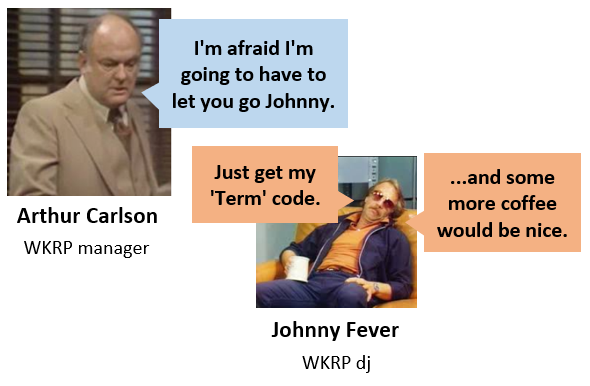
Johnny wants his term code so he can go home. Arthur’s data has several rows for the same person.
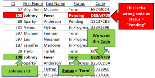
If he does a vlookup he’ll get the wrong term code (vlookup returns the first match it finds).
Get my Excel file and follow along.
Helper Column Solution
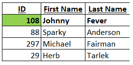
Here is the list of employees that Mr Carlson needs to terminate.
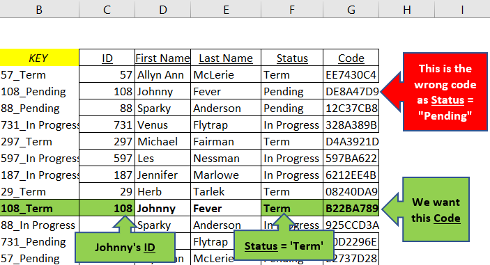
Sheet ‘new data’ has multiple rows for the same employee (with different Status codes). I created a helper formula in column B to concatenate ID and Status.
This is the formula =C5&”_”&F5 I used in column B. I could also use CONCATENATE function.
The formula below looks into column B to find the key and returns the Code (column G).
=INDEX(‘new data’!$G$5:$G$31,MATCH(D11&”_”&”Term”,’new data’!$B$5:$B$31,0))
This formula is added beside the list of employees that Mr Carlson needs to terminate.
My file lists solution steps in more detail. Read the next section to see what I should’ve done first!
Know Your Data!!
I made a dangerous assumption: What if there’s more than 1 row per person with a Status of ‘Term’ ? Which one is correct?
Below, COUNTIFS function in column H (Verify) counts the rows for each ID with a Status of ‘Term’.
=COUNTIFS(‘new data’!$C$5:$C$32,$D11,’new data’!$F$5:$F$32,”Term”)
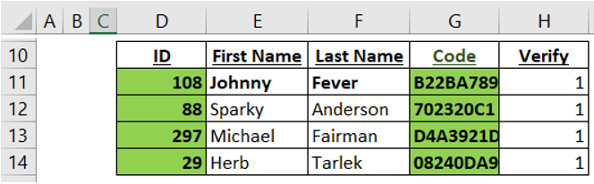
The result is 1 for each terminated employee so we can assume that the data is clean.
Array Formula Solution
If you don’t want to use a helper column then we can solve this using a single array formula.
=INDEX(‘new data’!$G$5:$G$31,MATCH(D11&”_”&$F$7,’new data’!$C$5:$C$31&”_”&’new data’!$F$5:$F$31,0))
To enter the above formula hold ‘Control’ & ‘Shift’ keys and then press ‘Enter’. Arrays takes time to learn but they can answer complex questions in a single formula.
Real Case
This was a real case from someone I know who needed help. She was spending an hour or two every month searching through data to find the correct code. Often when working with data there’s a missing concept that would make the task so much easier. In this case it was the concatenated key concept. It takes some time to learn a new concept but then your Excel skills become stronger and you can complete your work quicker.
It was also important to use Excel’s COUNTIFS function to confirm the assumption that each terminated employee only had 1 row with Status ‘Term’. If someone had two rows with Status ‘Term’ then that would be a problem (which one is correct?).
Update!
Arthur Carlson rehired Johnny and then had to fire Johnny a 2nd time. How can we retrieve Johnny’s last (most current) term code?
Robert H. Gascon added a comment below with this formula:
=LOOKUP(3,2/((‘new data’!$C$5:$C$35=$D11)*(‘new data’!$F$5:$F$35=”Term”)),’new data’!$G$5:$G$35)
It works nicely to give us the last term code for Johnny now that he has two term codes. Download the Excel file.
Thanks Robert!
About Me
My name is Kevin Lehrbass. I live in Markham Ontario Canada. I’ve been a Data Analyst since 2001.
I this post I used these functions: INDEX, MATCH, COUNTIFS. VLOOKUP could be used instead of INDEX MATCH.
These are some of the most common and useful functions in Excel. Once you know COUNTIFS then SUMIFS and AVERAGEIFS are easy.
Hello Kevin,
I added entries for Johnny Fever, Sparky Anderson, Michael Fairman, and Herb Tarlek to the new data Sheet, all with Term status and Code with the formula =”ABCDE”&TEXT(C32,”000″).
To return the last match, which I presume is the correct match, my formula is:
=LOOKUP(3,
2/((‘new data’!$C$5:$C$35=$D11)*(‘new data’!$F$5:$F$35=$F$7)),
‘new data’!$G$5:$G$35)
To return the first match, if it is presumed as correct, my formula is:
=LOOKUP(3,
2/(1/ROW(‘new data’!$F$5:$F$35)=MAX(INDEX(
1/ROW(‘new data’!$F$5:$F$35)*(‘new data’!$C$5:$C$35=$D11)*(‘new data’!$F$5:$F$35=$F$7),0))),
‘new data’!$G$5:$G$35)
As always, I used my favorite LOOKUP function along with the MAX-INDEX combination, being my resoundingly next favorite.
Hi Robert,
Very cool! We could create a scenario in which Johnny Fever gets fired, rehired and fired again! If the data is sorted by date (earliest at top to latest at the bottom) then your formula saves the day for manager Arthur Carlson! I’m going to update my post with your idea!
Thanks for reading and for the great formula idea Robert! Happy New Year!
Cheers,
Kevin
Hi Kevin,
Thanks for your compliment, Kevin. Your creative ideas inspire me to devise seemingly impossible formulas. My favorite is the LOOKUP function because I always LOOK UP to Him Above, when I am looking for a clever formula to solve your excellent challenges.
Cheers,
Robert
Pingback: Countifs confirms Vlookup | My Spreadsheet Lab
Pingback: Excel Chess Games Viewer | My Spreadsheet Lab