


Data lands in Microsoft Excel in many different structures. Data Analysts like me will often tell you to normalize your data before starting your analysis. This post contains three examples in which normalizing your data might not be necessary when doing a quick analysis.
Normalized Data?
Data is normalized when each column is a separate piece of information (i.e. column A is ‘Name’, column B is ‘Sales’, etc) and each row is a record or transaction (a row could potentially be an employee or a sales transaction).
Why Normalize?
It’s often best to normalize because Pivot Tables require this structure as do most formulas. However, we aren’t always building a long term efficient solution. Sometimes we are just answering a quick question and we may never use the data-set again.
Three Examples
Let’s take a look at three examples of non-normalized data and the questions that we have to answer.
Challenge #1
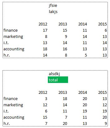
We need to add numbers for each Department & Year combination only when the word “total” appears in the header text of each pivoted block of data (there are many of these).
In the pic below, we would ignore the values from the 1st block of data and include the data from the 2nd block as the word “total” is found above the data.
Challenge #2
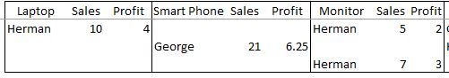
Get the average for ‘Sales’ and ‘Profit’ for Herman and George (data-set is wider making it challenging to do manually).
Challenge #3
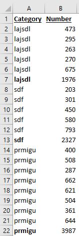
This one is a bit different. The data is normalized but the totals are included in the data (last item in each sorted group). How can we extract the last item?
Challenge #1 Solution
Modeloff champion Diarmuid Early reminded me of this technique several months ago.
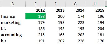
In the summary table seen below, we can use this formula in cell E2 =SUMIFS(E13:E651,$D13:$D651,$D2,$F$10:$F$648,”Total”) and then drag it to the right and down.
Leave the formula ranges locked and unlocked exactly the way they are for it to work! It only works because the department and year values are in the exact same order in each mini table.
Challenge #2 Solution
This formula solution =SUMIF($B$4:$Q$6,$B12,C$4:R$6) is similar. Note how columns C and R will slide over when dragged to the right! When the formula is dragged down only the row reference changes ($B12 becomes $B13).
Challenge #3 Solution
And finally we have (at least) two options for solving this. We could use an array =SMALL(IF($A$2:$A$22<>$A$3:$A$23,ROW($A$2:$A$22),””),I2) to get the row number of the last item (don’t forget to press ‘Control’ ‘Shift’ ‘Enter’ instead of just ‘Enter’) along with this index function =INDEX($B$1:$B$22,J2) to get the answer.
Alternatively, in this case, we know that the total is adding up all the values above that are in the same group. So, we could just do a SUMIF for each unique category and divide by 2.
Get My Excel File & Watch My Video
Download my Excel file here or from my OneDrive (file 00167). Watch my YouTube video.
About Me
I’ve worked with data since 2001. Discovering new techniques is a fun part of being a Data Analyst. I was going to add a 2nd caption saying “I’m going dancing” but most Data Analysts wouldn’t do that because moving on to the next data challenge would be more exciting!
