


Sometimes life is stranger than fiction. If we were to create this requirement as a hypothetical case many would say that it would never happen. Well, this was a real question that someone had for me. Read this post to see the requirements and how I solved this. I’ve also included alternative solutions from the Excel community.
Requirement
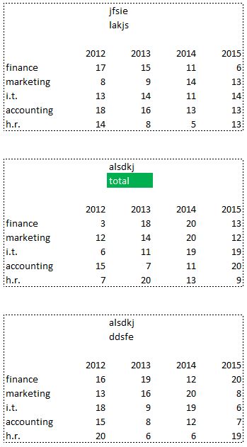
We have thousands of these non normalized mini ranges or groups of data stacked on top of each other. It’s always the same number of spaces between the groups.
We need to sum the numbers for each combination of business unit and year. Here’s the twist! We only sum the numbers from the groups of data that have “total” as the second title word!
The good news is that the business units are always in the same vertical order and the years are in the same left to right order.
Ask Some Questions Before Solving This!
Before we start writing formulas or vba code we really should ask a couple of questions that will determine how we solve this:
- Is this a quick one time task or a long term project?
- Does your co-worker or client want/need to understand the solution?
Now Let’s Look At Some Possible Solutions
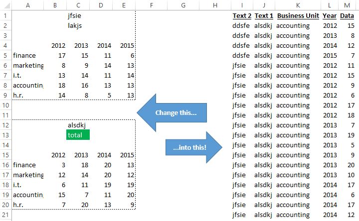
1. Normalize & Pivot Table
This is a good method if it’s a long term project that will have additional questions. In this case it’s worth the time to normalize that data and then use simple Pivot Tables or formulas. It would also be easy to add helper formula columns. Re-arranging or normalizing the data into a database format makes the analysis so much easier!
2. Helper Column and Sumifs
If this is a quick one time task then maybe it’s not worth spending the time to re-arrange/normalize the data. We can create a very simple helper column that will repeat the second text word.
Then, in cell E2, we use this formula =SUMIFS(E$13:E$655,$B$13:$B$655,”total”,$D$13:$D$655,$D2) drag it over and down and we are finished! Time for ice cream!

3. Array Formula!?!
For the brave at heart we can use a single array formula! No need to re-arrange the data or use a helper column.
This is our array formula–> =SUM(N(OFFSET(E$8,IFERROR(IF(($F$9:$F$655=”total”),ROW($C$9:$C$655)-ROW($C$9)+$C2,0),0),0)))
How does it work? Let’s look only at the OFFSET part for now.
OFFSET(E$8,IFERROR(IF(($F$9:$F$655=”total”),ROW($C$9:$C$655)-ROW($C$9)+$C2,0),0),0)
Remember that the mandatory arguments of an OFFSET function are: OFFSET(Reference, Rows, Cols) or is simple language OFFSET(starting cell, go down or up, go left or right)
This would normally return a single value. However, we know that in this case we need to return several values (a number from each table that has the word “total”). We need a way to put various numbers in OFFSET’s row argument (‘go down or up’).
So, we take our array condition IF(($F$9:$F$655=”total”) and each time we find the word “total” we use this ROW($C$9:$C$655)-ROW($C$9)+$C2 to give us all of the positions of the number we want in each table that has the word “total” just above it. Clear as mud? It would help if you watched my YouTube video on this and audited the file (see below).
4. Power Query!
Power Query (aka Get & Transform) is the hottest Excel tool since Pivot Tables!
Both Oz du Soleil and Piotr Majcher created Power Query solutions! Check out there videos!

Watch Piotr’s video!

Watch Oz’s video!
5. SUMIFS with a TWIST!

2014 MODELLOFF champion Diarmund Early left the comment below with a brilliant SUMIFS formula.

At first it looks like Diarmuid forget to lock the sum range and part of the criteria 1 range. Then I remembered that I used something similar to this several years ago! It’s a brilliant solution in the “One Time Task” category.
How does it work? The criteria 2 range that’s looking for “Total” is fully locked. the SUM range is not locked at all (rows nor columns). The formula is entered into cell E2 and then dragged down and to the right. Remember that the business units are always in the same order. The main logic to the formula is that the SUMIFS function is expecting ranges with the same number of items. The ranges are almost always parallel to each other but they don’t have to be! They just have to have the same number of elements. Isn’t Excel amazing!!!
Which Solution Is Best?
One Time Task: I’m going with Diarmuid Early’s SUMIFS solution! One simple non array quickly solves it! My helper/sumifs is a distant 2nd.
Long Term Project: Power Query wins! Oz du Soleil and Piotr Majcher convinced me! Using VBA to normalize is a decent 2nd prize.
Solution Contributors
A special thanks to Oz du Soleil (http://datascopic.net/), Piotr Majcher (http://www.pmsocho.com/) and Diarmuid Early (https://theexcelements.com/) for participating!
Excel File
Get the Excel file here (video 00160) or here.
YouTube Video
You can watch my YouTube video here.
About Me

My name is Kevin Lehrbass. I live in Markham, Ontario, Canada. I’ve been studying, supporting, building, troubleshooting, teaching and dreaming in Excel since 2001. I’m a Data Analyst.
There are so many amazing things that you can do with this powerful software. Check out my videos and my blog posts.
Away from Excel I enjoy playing with my dogs Cali & Fenton, learning Spanish and playing Chess.
Here’s another approach – enter this formula in cell E2 and copy down and to the right:
=SUMIFS(E13:E651,$D13:$D651,$D2,$F$10:$F$648,”Total”)