


Such a clear question originating from the classic: “How many unique items per group“?

Mike Girvin (ExcelIsFun) created several videos explaining different ways to solve this. See a couple of my ideas further down.
Let’s Take A Look At The Sample Data.
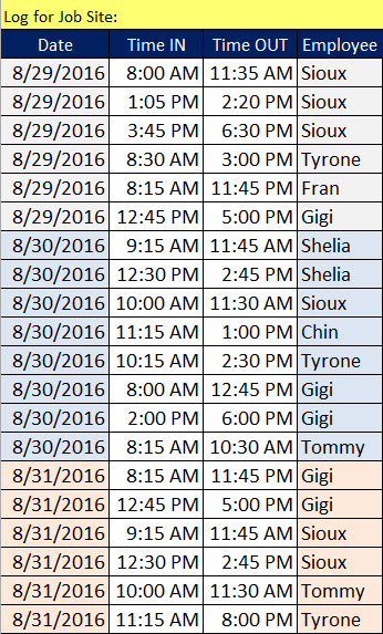
With this small sample we see that:
- 8/29/2016 has 4 unique visitors
- 8/30/2016 has 6 unique visitors
- 8/31/2016 has 4 unique visitors
Note that ‘Time IN’ and ‘Time OUT’ columns aren’t required for solving our question.
What’s The Best Way To Solve This?
My doodle below summarizes Mike’s solutions. Further down you’ll see my helper column solution and an alternative array formula solution.

What About A Simple PIVOT TABLE?
Data Model Solution
A traditional Pivot Table can’t solve this because there’s no distinct count function. The count function counts all employees per date including the duplicates. However, when creating a new Pivot Table we can check “Add this data to the Data Model” which displays a Distinct Count function!
Watch Mike Girvin’s video
Pivot Built On Pivot Solution
This sounds a bit odd but it’s a super fast method to solve our unique items per group question. Mike got the idea from Bill Szysz video .
GET & TRANSFORM?
Get & Transform is an amazing data tool! It is a built-in feature in Excel 2016 (add-in in Excel 2010 and 2013) that allows you to re-arrange your data. Watch Mike’s video to see how easy it is to solve the unique items per group question.
What About FORMULA Solutions?
If your data changes a Pivot Table solution requires a data refresh but formulas do not! This is an advantage but formula based solutions are more complex. Think of formula solutions as ‘cooking from scratch’ while Pivots are like packaged quick meals with little prep.
Array Formulas

Watch my entire YouTube video or only the method that you’re interested in below.
Method 1: Quick & Dirty REMOVE DUPLICATES

If you only have a few records then consider using Excel’s Remove Duplicates feature (YouTube).
Methods 2 & 3: Combine Helper Column with Sumif or Countif

Method 2: If arrays make you queasy and you don’t want to refresh a Pivot Table then consider a helper column with a simple formula like this =1/COUNTIFS($A$7:$A$26,A7,$D$7:$D$26,D7) followed by a Sumifs function (YouTube Video).
Method 3: This method uses three helper columns (a counter, a concatenated key and a match function) followed by a Countifs function (YouTube Video).
Method 4: Array Formula

So…I wondered if I could take the 1/COUNTIFS helper column idea and convert it into a single cell array formula. Eventually I got this to work and gave myself a high five! My dog Cali didn’t seem to be impressed.
My Array Formula:
=SUM(IFERROR(1/COUNTIFS($A$7:$A$26,K7,$A$7:$A$26,$A$7:$A$26,$D$7:$D$26,$D$7:$D$26),0))
Mike’s Array Formula:
=SUM(IF(FREQUENCY(IF($D$7:$D$26<>””,IF($A$7:$A$26=K7,MATCH($D$7:$D$26,$D$7:$D$26,0))),ROW($D$7:$D$26)-ROW($D$6)),1))
Are You Falling In Love With Array Formulas?
If so, there’s one thing that you have to do: BUY MIKE’S BOOK!
About Me
 My name is Kevin Lehrbass. This is my personal blog about Microsoft Excel. I live in Markham, Ontario, Canada. I’ve been studying, supporting, building, troubleshooting, teaching and dreaming in Excel since 2001. I’m a Data Analyst.
Thousands of hours can be saved and costly errors can be avoided or corrected if you study this powerful software. Check out my videos and blog posts.
Away from Excel I enjoy playing with my dog Cali, learning Spanish, playing Chess and drawing nerds.
Hello Kevin,
You really deserve a high five for your succinct formula! As a non-array alternative, I suggest this formula:
=SUMPRODUCT(–(FREQUENCY(COUNTIF(D$7:D$26,”>=”&D$7:D$26)*(A$7:A$26=K7),
COUNTIF(D$7:D$26,”>=”&D$7:D$26)*(A$7:A$26=K7))>0))-1
Cheers,
Robert
Excellent formula! Thanks Robert!